Introduction
This document outlines the approach i took to download data level 3 TCGA data. RNA-seq, methylation 450K data and clinical information was downloaded using the RTCGAToolbox(Samur 2014) package
The RTCGAToolbox package written by Samur, retreives data from the broads institutive firehose database. Detailed information on how to use this package are available in the Vignette, online courses PH525Xseries and Youtube videos. Many of the codes used here were taken from these resources.
#Load the library
library(RTCGAToolbox)
A list of available cancer types are found using the getFirehoseDatasets command. The run dates and analyze datas are found using the getFirehoseRunningDates and the getFirehoseAnalyzeDates commands.
getFirehoseDatasets()## [1] "ACC" "BLCA" "BRCA" "CESC" "CHOL" "COADREAD"
## [7] "COAD" "DLBC" "ESCA" "FPPP" "GBMLGG" "GBM"
## [13] "HNSC" "KICH" "KIPAN" "KIRC" "KIRP" "LAML"
## [19] "LGG" "LIHC" "LUAD" "LUSC" "MESO" "OV"
## [25] "PAAD" "PCPG" "PRAD" "READ" "SARC" "SKCM"
## [31] "STAD" "STES" "TGCT" "THCA" "THYM" "UCEC"
## [37] "UCS" "UVM"head(getFirehoseRunningDates())## [1] "20160128" "20151101" "20150821" "20150601" "20150402" "20150204"head(getFirehoseAnalyzeDates())## [1] "20160128" "20150821" "20150402" "20141017" "20140715" "20140416"Clinical and RNA-seq data - download and process
The clinical information and normalised RNA-seq data is downloaded. The methylation data is downloaded separately from the clinical and RNA-seq data because its size was too large for my computer to handle. Thus the methylation data was downloaded in separately in our University departments computer cluster.
Skin cutaneous melanoma (SKCM) is selected and “20160128” is used as the rundate. The default file size is 500 mb and this limit is extended to 3000 mb using fileSizeLimit.
The RNA-seq data (RNASeq2GeneNorm) contains normalised gene expression levels generated using MapSplice for alignment and RNA-Seq by Expectation-Maximization (RSEM) for quantification. RSEM values are calculated using an algorithm that estimate abundances at the gene level to generate TPM (Transcripts Per Million) values. TPM is similar to FPKM and RPKM in that it accounts for total number of reads and gene length. However TPM has gained more popularity over recent years because it is easier to interpret and more stable when comparing between samples. The normalisation is done by dividing the TPM values by the 75th percentile (3rd quartile) and multiplication by 1000.
readDataSKCM <- getFirehoseData (dataset="SKCM",
                                runDate="20160128",
                                forceDownload = TRUE,
                                clinical = TRUE,
                                RNASeq2GeneNorm = TRUE,
Methylation = FALSE, fileSizeLimit= 3000)load("~/Dropbox/GitHub/Downloading-TCGA-data/RDatafiles/TCGA_readDataSKCM.RData")#extract the data
clinSKCM <- getData(readDataSKCM, "clinical")
rnaseqSKCM <- getData(readDataSKCM, "RNASeq2GeneNorm")The clinical and RNA-seq data are processed (or cleaned up) before any downstream analysis.
The TCGA barcodes are structured differently between the clinical and RNA-seq datasets and thus needs to be matched. For example the first TCGA barcode in the RNAseq data is “TCGA-3N-A9WB-06A-11R-A38C-07” whereas in the clinical data it is “tcga.d3.a2je”
Some samples have 2x RNA-seq data. Duplicate RNA-seq data are removed.
Some samples contain RNA-seq data but there is no clinical information. Only those samples that have both RNA-seq and clinical information are retained for downstream analysis.
#Changing patient identifier names
dim(clinSKCM)
## [1] 470 18head(clinSKCM)## Composite Element REF years_to_birth vital_status
## tcga.d3.a2je value 75 1
## tcga.d3.a2jf value 74 0
## tcga.d3.a3c8 value 58 0
## tcga.d3.a3ml value 70 1
## tcga.d3.a51g value <NA> 0
## tcga.d3.a8gi value 68 1
## days_to_death days_to_last_followup
## tcga.d3.a2je 841 <NA>
## tcga.d3.a2jf <NA> 1888
## tcga.d3.a3c8 <NA> 1409
## tcga.d3.a3ml 422 <NA>
## tcga.d3.a51g <NA> <NA>
## tcga.d3.a8gi 1780 <NA>
## days_to_submitted_specimen_dx pathologic_stage
## tcga.d3.a2je 140 stage iiic
## tcga.d3.a2jf 544 stage ia
## tcga.d3.a3c8 0 stage iiic
## tcga.d3.a3ml 230 stage iiia
## tcga.d3.a51g <NA> stage 0
## tcga.d3.a8gi 1653 stage ia
## pathology_T_stage pathology_N_stage pathology_M_stage
## tcga.d3.a2je tx n3 m0
## tcga.d3.a2jf t1a n0 m0
## tcga.d3.a3c8 tx n3 m0
## tcga.d3.a3ml t3a n2a m0
## tcga.d3.a51g tis n0 m0
## tcga.d3.a8gi t1a n0 m0
## melanoma_ulceration melanoma_primary_known Breslow_thickness
## tcga.d3.a2je <NA> yes <NA>
## tcga.d3.a2jf no yes 0.28
## tcga.d3.a3c8 <NA> yes <NA>
## tcga.d3.a3ml no yes 2.3
## tcga.d3.a51g <NA> yes 0
## tcga.d3.a8gi no yes 0.98
## gender date_of_initial_pathologic_diagnosis radiation_therapy
## tcga.d3.a2je female 2009 no
## tcga.d3.a2jf male 2008 no
## tcga.d3.a3c8 female 2009 yes
## tcga.d3.a3ml male 2003 no
## tcga.d3.a51g male <NA> no
## tcga.d3.a8gi male 2008 no
## race ethnicity
## tcga.d3.a2je white not hispanic or latino
## tcga.d3.a2jf white not hispanic or latino
## tcga.d3.a3c8 white not hispanic or latino
## tcga.d3.a3ml white not hispanic or latino
## tcga.d3.a51g white not hispanic or latino
## tcga.d3.a8gi white not hispanic or latinodim(rnaseqSKCM)## [1] 20501 473rnaseqSKCM[1:5,1:5]## TCGA-3N-A9WB-06A-11R-A38C-07 TCGA-3N-A9WC-06A-11R-A38C-07
## A1BG 381.0662 195.1822
## A1CF 0.0000 0.0000
## A2BP1 0.0000 0.0000
## A2LD1 250.1979 160.7548
## A2ML1 7.2698 0.0000
## TCGA-3N-A9WD-06A-11R-A38C-07 TCGA-BF-A1PU-01A-11R-A18S-07
## A1BG 360.8794 176.3994
## A1CF 0.7092 0.0000
## A2BP1 6.3830 1.2987
## A2LD1 97.1986 163.2338
## A2ML1 0.0000 7.7922
## TCGA-BF-A1PV-01A-11R-A18U-07
## A1BG 216.8470
## A1CF 0.0000
## A2BP1 0.0000
## A2LD1 60.8727
## A2ML1 0.5977#The identifiers in the RNA-seq data are transformed to be the same as the ones in the clinical data. This includes substringing the first 12 characters and replacing "-" with "."
rid = tolower(substr(colnames(rnaseqSKCM),1,12))
rid = gsub("-", ".", rid)
colnames(rnaseqSKCM) = rid
length(intersect(rid,rownames(clinSKCM))) # 469 samples intersect between RNAseq and clinSKCM## [1] 469#Remove duplicated samples
#Samples with duplicated names are removed. The data between the replicates are very similar however looking into the original barcodes, some of the duplicates are primary or metastatic, or a normal solid tumour. Tumours that are labeled primary, normal solid tumour or additional metastatic are removed.
duplicatedSamples <- which(duplicated(colnames(rnaseqSKCM))) # 4 duplicate samples
duplicatedSampleNames <- colnames(rnaseqSKCM)[duplicated(colnames(rnaseqSKCM))]
rnaseqMel_duplicated <- rnaseqSKCM[,colnames(rnaseqSKCM) %in% duplicatedSampleNames] #matrix of only those duplicated samples
colnames(rnaseqMel_duplicated)## [1] "tcga.d3.a1qa" "tcga.d3.a1qa" "tcga.er.a19t" "tcga.er.a19t"
## [5] "tcga.er.a2nf" "tcga.er.a2nf" "tcga.gn.a4u8" "tcga.gn.a4u8"par(mfrow=c(2,2))
plot(log2(rnaseqMel_duplicated[1001:2000,1:2]))
plot(log2(rnaseqMel_duplicated[1001:2000,3:4]))
plot(log2(rnaseqMel_duplicated[1001:2000,5:6]))
plot(log2(rnaseqMel_duplicated[1001:2000,7:8]))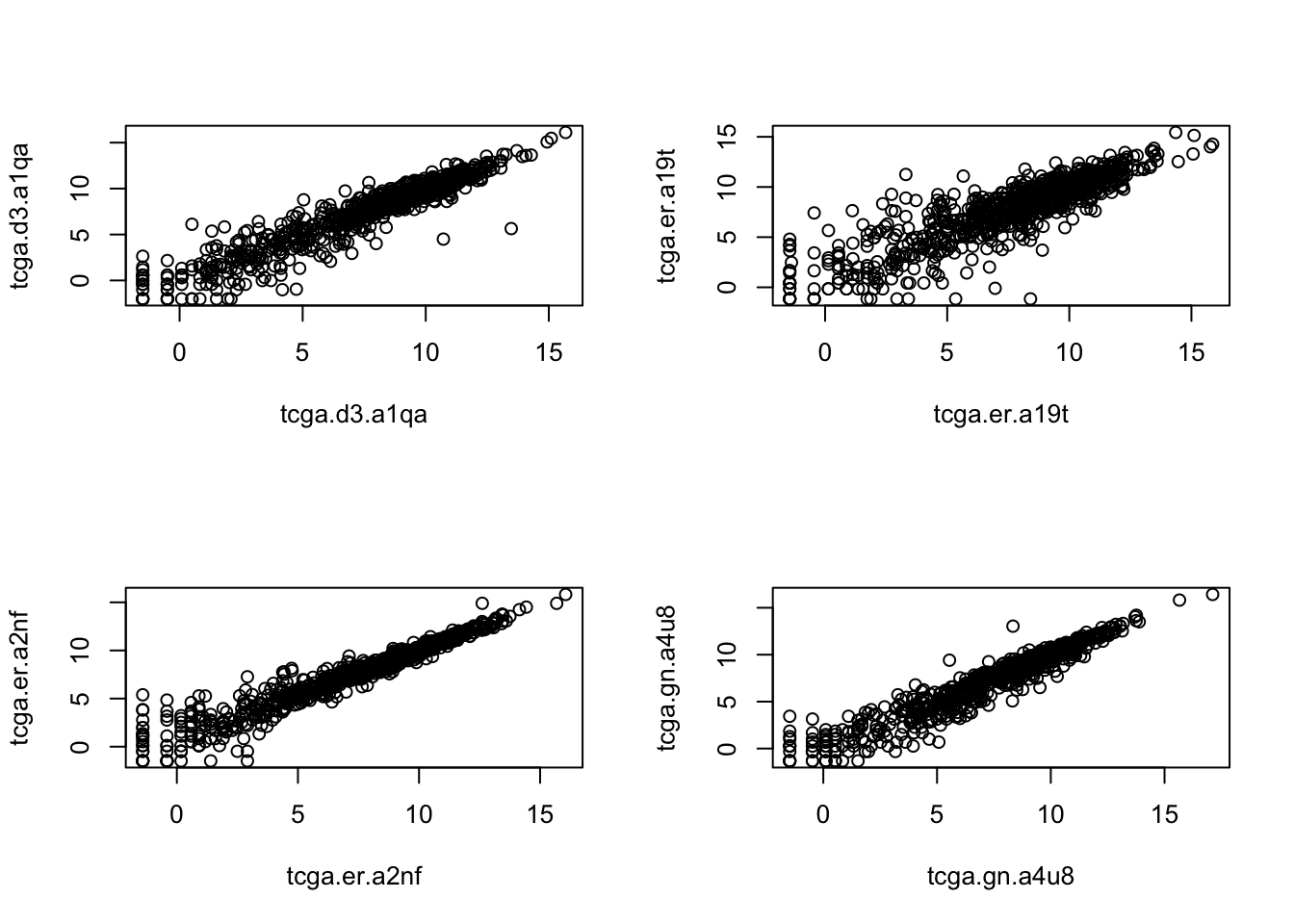
Figure 1: figure1:The duplicate samples are plotted together to assess the correlation. They look similar and it is not obvious which duplicate to keep.
The full TCGA barcodes names of these duplicate samples are investigated. Information on TCGA barcodes are given here and information on the sample type (e.g. primary, metastatic, additional metastsatic) from the TCGA barcode is provided here.
index <- which(colnames(rnaseqSKCM) %in% duplicatedSampleNames)

rnaseqSKCM2 <- getData(readDataSKCM, "RNASeq2GeneNorm")
original_rnaseq_barcode <- colnames(rnaseqSKCM2)
original_rnaseq_barcode[index]
## [1] "TCGA-D3-A1QA-07A-11R-A37K-07" "TCGA-D3-A1QA-06A-11R-A18T-07"
## [3] "TCGA-ER-A19T-06A-11R-A18U-07" "TCGA-ER-A19T-01A-11R-A18T-07"
## [5] "TCGA-ER-A2NF-06A-11R-A18T-07" "TCGA-ER-A2NF-01A-11R-A18T-07"
## [7] "TCGA-GN-A4U8-11A-11R-A32P-07" "TCGA-GN-A4U8-06A-11R-A32P-07"The sample types of these duplicate samples are either of primary solid (01) tumour, metastastic (06), additional metastastic (07) or solid tissue (11) normal.
Here, from the duplicates, i will retain only metastatic tumours and so I remove the duplicate primary solid tumours, additional metastatic tumour and solid tissue normal. 1st duplicate samples: remove the additional metastatic 2nd duplicate samples: remove the primary tumour 3rd duplicate samples: remove the primary 4th duplicate samples: remove the solid tissue normal
remove_index <- c("TCGA-D3-A1QA-07A-11R-A37K-07", "TCGA-ER-A19T-01A-11R-A18T-07",  "TCGA-ER-A2NF-01A-11R-A18T-07", "TCGA-GN-A4U8-11A-11R-A32P-07") #excluding these

remove_index <- which(original_rnaseq_barcode %in% remove_index)

rnaseqSKCM = rnaseqSKCM[,-remove_index] # getting rid of the duplicate

dim(rnaseqSKCM) # from 473 samples to 469
## [1] 20501 469length(intersect(colnames(rnaseqSKCM),rownames(clinSKCM))) #469 samples interect between rnaseqSKCM and clinSKCM## [1] 469length(rownames(clinSKCM)) # there is 1 sample in clinMel which there is absent in rnaseqMel ## [1] 470clinSKCM <- clinSKCM[intersect(colnames(rnaseqSKCM),rownames(clinSKCM)),]
dim(clinSKCM)## [1] 469 18table(colnames(rnaseqSKCM)==rownames(clinSKCM)) # patient names are in the same order##
## TRUE
## 469#You may wish to create an expression set which contains both RNA-seq and expression matrix.
library(Biobase)
readES = ExpressionSet(as.matrix(log2(rnaseqSKCM+1)))
pData(readES) = clinSKCMSurvival data clean-up and analysis
Survival analysis: background
To analyse overall survival, 3 variables in the clinMel data set is required, which are “vital_status”, “days_to_death” and “days_to_last_followup”.
Information is available in a googles forum page here
dim(clinSKCM)## [1] 469 18str(clinSKCM[,c("vital_status","days_to_death","days_to_last_followup")])## 'data.frame': 469 obs. of 3 variables:
## $ vital_status : chr "1" "0" "1" "0" ...
## $ days_to_death : chr "518" NA "395" NA ...
## $ days_to_last_followup: chr NA "2022" NA "387" ...clinSKCM[1:5,c("vital_status","days_to_death","days_to_last_followup")]## vital_status days_to_death days_to_last_followup
## tcga.3n.a9wb 1 518 <NA>
## tcga.3n.a9wc 0 <NA> 2022
## tcga.3n.a9wd 1 395 <NA>
## tcga.bf.a1pu 0 <NA> 387
## tcga.bf.a1pv 0 <NA> 14- vital_status: “1” means deceased and “0” means still alive.
- days_to_death: With patients who are deacesed, the days_to_death variable gives the number of days before death.
- days_to_last_followup: With patients who are still alive, the days_to_last_followup variable gives the number of days before the last follow-up.
Survival data: Exploratory analysis
In 460 out of 469 patients, the days_to_death and days_to_last_followup are mutually exlcusive; if theres an NA in days_to_death then there is a number to DaystoLastfollowup and vice versa. The remaining have NA for both days_to_death and days_to_last_followup.
table(!is.na(clinSKCM[,"days_to_death"]) & is.na(clinSKCM[,"days_to_last_followup"])) #There are 220 patients who does not contain (NA) days_to_last_followup however contains days_to_death##
## FALSE TRUE
## 249 220table(is.na(clinSKCM[,"days_to_death"]) & !is.na(clinSKCM[,"days_to_last_followup"])) #There are 240 patients that do not contain (NA) days_to_death but contain days_to_last_followup##
## FALSE TRUE
## 229 240table(is.na(clinSKCM$"days_to_death") & is.na(clinSKCM$"days_to_last_followup")) #there are 9 patinets that contain NA for both days_to_death and days_to_last_followup##
## FALSE TRUE
## 460 9There are 9 patients with both “days_to_death” and “days_to_last_followup” as NA.
survivalVariables <- c("days_to_last_followup","vital_status","days_to_death")

index <- is.na(clinSKCM[,"days_to_death"]) & is.na(clinSKCM[,"days_to_last_followup"])
clinSKCM[index,survivalVariables]
## days_to_last_followup vital_status days_to_death
## tcga.d3.a3c1 <NA> 0 <NA>
## tcga.d3.a3c3 <NA> 0 <NA>
## tcga.d3.a51g <NA> 0 <NA>
## tcga.d3.a8go <NA> 1 <NA>
## tcga.er.a19o <NA> 1 <NA>
## tcga.fr.a3yo <NA> 0 <NA>
## tcga.rp.a695 <NA> 0 <NA>
## tcga.rp.a6k9 <NA> 0 <NA>
## tcga.yd.a9tb <NA> 0 <NA>dim(clinSKCM[index,survivalVariables])## [1] 9 3There is also 1 patient with a negative days_to_last_followup. What does this mean?
survivalVariables <- c("days_to_last_followup","vital_status","days_to_death")

index <- which(clinSKCM[,"days_to_death"] < 0 | clinSKCM[,"days_to_last_followup"] < 0)

clinSKCM[index,survivalVariables]
## days_to_last_followup vital_status days_to_death
## tcga.eb.a430 -2 0 <NA>Survival analysis: merge days_to_death and days_to_last_followup
Here i merge days_to_death and days_to_last_followup to create a new variable called new_death. Most are simple to handle because they are mutually exlcusive; if there’s an NA in days_to_death then there is a number to days_to_last_followup and vice versa.
DELETE: However, as shown above, some patients have values to both variables with different number of days which i am unsure what that means. Also some patients have an NA to both variables.
Here i create a new variable called new_death in which: * If patient has deceased (1 in vital status), the days_to_death is selected * If patient is alive (0 in vital status), days_to_last_followup is selected
mergeOS <- ifelse(clinSKCM[,"vital_status"]==1, clinSKCM[,"days_to_death"], clinSKCM[,"days_to_last_followup"] )

str(mergeOS)
## chr [1:469] "518" "2022" "395" "387" "14" "282" "853" "831" "464" ...table(is.na(mergeOS))##
## FALSE TRUE
## 460 9clinSKCM$mergeOS <- as.numeric(mergeOS)Survival analysis: sanity check with t-stage
Here i perform a “sanity check” to see if the survival data makes sense. First i look at the prognosis according to the tumour T stage.
- t0 - patients without a known primary tumor.
- t1 - melanoma is less than 1 mm thick
- t2 - melanoma is between 1 mm and 2 mm thick
- t3 - melanoma is between 2 mm and 4 mm thick
- t4 - melanoma is more than 4 mm thick
- tis - Melanoma in situ
- tx - Primary tumor cannot be assessed (e.g. severely regressed melanoma or curettaged melanoma)
library(survival)ev <- as.numeric(clinSKCM$vital_status)
fut <-as.numeric(clinSKCM$mergeOS)
su = Surv(fut, ev)
# There are 15 different types of T-stage. Here i reduce this number to 7 different groups.
table(clinSKCM$pathology_T_stage)##
## t0 t1 t1a t1b t2 t2a t2b t3 t3a t3b t4 t4a t4b tis tx
## 23 10 22 10 32 31 15 14 39 37 15 25 112 8 47table(substr(clinSKCM$pathology_T_stage,1,2)) ##
## t0 t1 t2 t3 t4 ti tx
## 23 42 78 90 152 8 47t_stage = factor(substr(clinSKCM$pathology_T_stage,1,2))plot(survfit(su~t_stage),mark.time=TRUE, lwd=2, col=1:7, las=1, cex.axis=1.5)
mtext("Overall Survival", side=2, line=2.7, cex=1.5)
mtext("Time (Days)", side=1, line=2.8, cex=1.5)
ntab = table(t_stage)
ns = paste("[n=", ntab, "]", sep="")
legend(8000, .95, col=1:7, lwd=2, legend=paste(levels(t_stage), ns))
text(6000,1, paste("p.value = 5.25e-06"))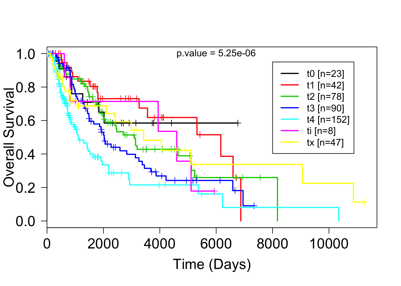
Figure 2: figure2:Kaplan Meier survival plot of melanoma patients in the TCGA databse according to T stage. As expected, survival becomes poorer from t1 to t4. However it is strange that ti (tis, melanoma insitu) has a sudden drop in survival.
summary(coxph(su~t_stage))## Call:
## coxph(formula = su ~ t_stage)
##
## n= 433, number of events= 205
## (36 observations deleted due to missingness)
##
## coef exp(coef) se(coef) z Pr(>|z|)
## t_staget1 -0.1524 0.8586 0.4383 -0.348 0.72803
## t_staget2 0.2414 1.2730 0.3876 0.623 0.53351
## t_staget3 0.5201 1.6822 0.3816 1.363 0.17289
## t_staget4 1.0727 2.9231 0.3759 2.854 0.00432 **
## t_stageti 0.3821 1.4654 0.5718 0.668 0.50394
## t_stagetx 0.2102 1.2340 0.4250 0.495 0.62084
## ---
## Signif. codes: 0 '***' 0.001 '**' 0.01 '*' 0.05 '.' 0.1 ' ' 1
##
## exp(coef) exp(-coef) lower .95 upper .95
## t_staget1 0.8586 1.1646 0.3637 2.027
## t_staget2 1.2730 0.7856 0.5955 2.721
## t_staget3 1.6822 0.5945 0.7963 3.554
## t_staget4 2.9231 0.3421 1.3993 6.106
## t_stageti 1.4654 0.6824 0.4778 4.494
## t_stagetx 1.2340 0.8104 0.5364 2.839
##
## Concordance= 0.624 (se = 0.023 )
## Rsquare= 0.071 (max possible= 0.992 )
## Likelihood ratio test= 31.92 on 6 df, p=2e-05
## Wald test = 32.6 on 6 df, p=1e-05
## Score (logrank) test = 34.56 on 6 df, p=5e-06survdiff(su~t_stage)## Call:
## survdiff(formula = su ~ t_stage)
##
## n=433, 36 observations deleted due to missingness.
##
## N Observed Expected (O-E)^2/E (O-E)^2/V
## t_stage=t0 23 8 12.7 1.7284 1.8504
## t_stage=t1 42 15 27.4 5.5960 6.5269
## t_stage=t2 76 40 49.4 1.7855 2.3821
## t_stage=t3 89 49 46.3 0.1534 0.1996
## t_stage=t4 152 68 38.5 22.5570 29.1185
## t_stage=ti 7 5 5.3 0.0169 0.0175
## t_stage=tx 44 20 25.4 1.1457 1.4286
##
## Chisq= 34.6 on 6 degrees of freedom, p= 5e-06There is a significant statistical difference in overall survival between the different T stages.
It is strange that those patients with melanoma insitu has such a poor prognosis. Here i look at the clinical data of these patients. All 8 of these patients did not have distant metastsis and only 1 presented regional lymph node metastasis. However 5 ended up deceased.
clinSKCM[clinSKCM$pathology_T_stage %in% "tis",]## Composite Element REF years_to_birth vital_status
## tcga.d3.a2jb value 70 1
## tcga.d3.a51g value <NA> 0
## tcga.d3.a51k value 51 0
## tcga.d3.a8gr value 54 1
## tcga.ee.a183 value 48 1
## tcga.ee.a20c value 59 1
## tcga.ee.a29w value 42 0
## tcga.er.a2ne value 39 1
## days_to_death days_to_last_followup
## tcga.d3.a2jb 5110 <NA>
## tcga.d3.a51g <NA> <NA>
## tcga.d3.a51k <NA> 1002
## tcga.d3.a8gr 3943 <NA>
## tcga.ee.a183 818 <NA>
## tcga.ee.a20c 4601 <NA>
## tcga.ee.a29w <NA> 5932
## tcga.er.a2ne 613 <NA>
## days_to_submitted_specimen_dx pathologic_stage
## tcga.d3.a2jb 3035 stage 0
## tcga.d3.a51g <NA> stage 0
## tcga.d3.a51k 20 stage iiib
## tcga.d3.a8gr 3774 stage 0
## tcga.ee.a183 447 stage 0
## tcga.ee.a20c 4469 stage 0
## tcga.ee.a29w 4954 stage 0
## tcga.er.a2ne 567 stage 0
## pathology_T_stage pathology_N_stage pathology_M_stage
## tcga.d3.a2jb tis n0 m0
## tcga.d3.a51g tis n0 m0
## tcga.d3.a51k tis n2b m0
## tcga.d3.a8gr tis n0 m0
## tcga.ee.a183 tis n0 m0
## tcga.ee.a20c tis n0 m0
## tcga.ee.a29w tis n0 m0
## tcga.er.a2ne tis n0 m0
## melanoma_ulceration melanoma_primary_known Breslow_thickness
## tcga.d3.a2jb <NA> yes <NA>
## tcga.d3.a51g <NA> yes 0
## tcga.d3.a51k <NA> yes 0
## tcga.d3.a8gr <NA> yes 0.01
## tcga.ee.a183 <NA> yes <NA>
## tcga.ee.a20c <NA> yes <NA>
## tcga.ee.a29w <NA> yes 0
## tcga.er.a2ne <NA> yes <NA>
## gender date_of_initial_pathologic_diagnosis radiation_therapy
## tcga.d3.a2jb female 1997 no
## tcga.d3.a51g male <NA> no
## tcga.d3.a51k male 2011 no
## tcga.d3.a8gr female 1999 no
## tcga.ee.a183 male 2007 no
## tcga.ee.a20c male 1997 no
## tcga.ee.a29w male 1997 yes
## tcga.er.a2ne male 2007 yes
## race ethnicity mergeOS
## tcga.d3.a2jb black or african american not hispanic or latino 5110
## tcga.d3.a51g white not hispanic or latino NA
## tcga.d3.a51k white hispanic or latino 1002
## tcga.d3.a8gr white not hispanic or latino 3943
## tcga.ee.a183 white not hispanic or latino 818
## tcga.ee.a20c white not hispanic or latino 4601
## tcga.ee.a29w white not hispanic or latino 5932
## tcga.er.a2ne white not hispanic or latino 613Survival analysis: sanity check with CD74
Another “sanity check” is done but this time with using the RNAseq data. CD74 gene exprresion was found to be associated with good prognosis using SKCM TCGA data (Ekmekcioglu 2016).
#Patient samples are split into high and low CD74 expression using the median as the cut-off
CD74 <- ifelse(rnaseqSKCM["CD74",] > median(rnaseqSKCM["CD74",]), 1, 0)
# higher than median is 1, lower than median is 0
CD74 <- as.factor(CD74)
table(CD74)
## CD74
## 0 1
## 235 234ev <- as.numeric(clinSKCM$vital_status)
fut <-as.numeric(clinSKCM$mergeOS)
su = Surv(fut, ev)plot(survfit(su~CD74),mark.time=TRUE, lwd=2, col=c("black","red"), las=1, cex.axis=1.5)
mtext("Overall Survival", side=2, line=2.7, cex=1.5)
mtext("Time (Days)", side=1, line=2.8, cex=1.5)
ntab = table(CD74)
ns = paste("[n=", ntab, "]", sep="")
legend(6000, .8, col= c("black","red"), lwd=2, legend=paste(c("low CD74", "high CD74"), ns))
text(4000,0.8, paste("p.value= 1.94e-06"))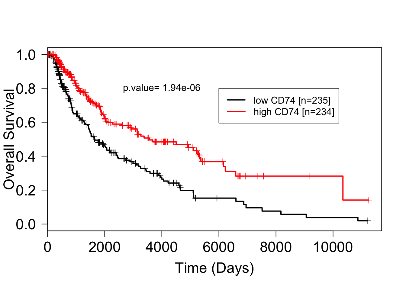
Figure 3: figure3:Kaplan Meier survival plot of melanoma patients in the TCGA databse according to high and low CD74 expression. Consistent with Ekmekcioglu2016, higher CD74 expression is associated with better prognosis.
survdiff(su~CD74, data=clinSKCM)## Call:
## survdiff(formula = su ~ CD74, data = clinSKCM)
##
## n=460, 9 observations deleted due to missingness.
##
## N Observed Expected (O-E)^2/E (O-E)^2/V
## CD74=0 230 133 98 12.5 22.7
## CD74=1 230 87 122 10.0 22.7
##
## Chisq= 22.7 on 1 degrees of freedom, p= 2e-06Methylation 450K data - download and processing
The methylation 450K data-frame was too big (>6gb) to download or work with in my desktop. It has 485,577 rows and 478 columns with each value having many digits. Therefore I had to use our cluster network to download the data and then reduce the file size by lowering the number of decimal points for every beta-value. The size-reduced file was then moved to my desktop and loaded into R.
#This was done in our DSM cluster
#downloading the methylation 450k data from TCGA melanoma samples
readDataSKCM_methylation <- getFirehoseData(dataset = "SKCM",
                               runDate = "20160128",
                               forceDownload = TRUE,
                               clinical = FALSE,
                               RNASeq2GeneNorm = FALSE,
                               Methylation = TRUE,
                               fileSizeLimit = 3000)

me450kSKCM = getData(readDataSKCM_methylation, "Methylation",1)
probeinfo <- me450kSKCM[,1:3]
me450kSKCM <- me450kSKCM[,-(1:3)]
me450kSKCM <- sapply(me450kSKCM, as.numeric)
save.image("methylation450k_20160128_raw.RData")
#scp /home/STUDENT/ahnje770/methylation450k_20160128_raw.RData /mnt/hcs/dsm-eccles-seq
names(as.list(.GlobalEnv)) #too look at the varialbes in the global environment (in the DSM cluster)
#to load it in the future in DSM cluster
load("/mnt/hcs/dsm-eccles-seq/methylation450k_files/methylation450k_20160128_raw.RData")Change the identifier names in the methylation data
rid = tolower(substr(colnames(me450kSKCM),1,12))
rid = gsub("-", ".", rid)

duplicatedSampleNames_me450k <- rid[which(duplicated(rid))]
colnames(me450kSKCM)[rid %in% duplicatedSampleNames_me450k]
# [1] "TCGA-D3-A1QA-07A-11D-A373-05" "TCGA-D3-A1QA-06A-11D-A19B-05"
# [3] "TCGA-ER-A19T-06A-11D-A19D-05" "TCGA-ER-A19T-01A-11D-A19D-05"
# [5] "TCGA-ER-A2NF-06A-11D-A19D-05" "TCGA-ER-A2NF-01A-11D-A19D-05"
# [7] "TCGA-FW-A3R5-11A-11D-A23D-05" "TCGA-FW-A3R5-06A-11D-A23D-05"
# [9] "TCGA-GN-A4U8-11A-11D-A32S-05" "TCGA-GN-A4U8-06A-11D-A32S-05"

#Just as the RNA-seq data, here I remove the additional metastatic, primary tumours, and normal solid tissues

#removing the duplicated samples here
#1st duplicate: remove the additional metastatic (07)
#2nd duplicate: remove the primary tumour (01)
#3rd duplicate: remove the primary (01)
#4th duplicate: remove the solid tissue normal (11)
#5th duplicate: remove the solid tissue normal (11)

#01 Primary solid tumour
#06 metastatic
#07 additional metastastatic
#11 Solid tissue normal

remove_index <- c("TCGA-D3-A1QA-07A-11D-A373-05", "TCGA-ER-A19T-01A-11D-A19D-05" ,  "TCGA-ER-A2NF-01A-11D-A19D-05", "TCGA-FW-A3R5-11A-11D-A23D-05", "TCGA-GN-A4U8-11A-11D-A32S-05")
remove_index <- which(colnames(me450kSKCM) %in% remove_index)
remove_index #the rows i will be removing for the duplicated samples
#[1]  36 316 324 387 414

me450kSKCM = me450kSKCM[,-remove_index] # getting rid of the duplicate

dim(me450kSKCM) # from 475 samples to 470
table(duplicated(colnames(me450kSKCM)))
#FALSE
#  470

rid = tolower(substr(colnames(me450kSKCM),1,12))
rid = gsub("-", ".", rid)

colnames(me450kSKCM) <- rid

length(intersect(colnames(me450kSKCM),colnames(rnaseqSKCM)))  #469 samples interect between meTIL_probes and rnaseqSKCM
length(colnames(meTIL_probes)) # there is 1 sample in clinMel which there is absent in rnaseqMel

me450kSKCM <- me450kSKCM[,intersect(colnames(me450kSKCM),colnames(rnaseqSKCM))]
dim(meTIL_probes)

table(colnames(rnaseqSKCM)==colnames(me450kSKCM)) # patient names are in the same order
Reducing the size of the methylation 450K data
str(me450kSKCM) # this shows that all the values are characters.

me450kSKCM <- sapply(me450kSKCM, as.numeric)
me450kSKCM_rounded <- as.matrix(round(me450kSKCM, digits=3)) # Round to 3 digits
write.csv(me450kSKCM_rounded, "me450kSKCM_rounded.csv")

#scp /home/STUDENT/ahnje770/me450kSKCM_rounded.csv /mnt/hcs/dsm-eccles-seq

rm(me450kSKCM) #remove the unrounded me450kfile
setwd("/mnt/hcs/dsm-eccles-seq/methylation450k_files")

save.image("methylation450k_20160128_rounded.RData")
After i reduced the size of the methylation data to generate me450kMel_rounded, I saved into my computer for loading.
load ("~/Dropbox/GitHub/RDatafiles/methylation450k_20160128_rounded.RData")

# load("/Volumes/dsm-eccles-seq/methylation450k_files/methylation450k_20160128_rounded.RData") #"/Volumes" (on my dekstop) is the same as "/mnt/hcs" (in DSM cluster)

dim(me450kSKCM_rounded)
## [1] 485577 469dim(probeinfo)## [1] 485577 3class(me450kSKCM_rounded)## [1] "matrix"me450kSKCM_rounded[1:3,1:3]## tcga.3n.a9wb tcga.3n.a9wc tcga.3n.a9wd
## cg00000029 0.517 0.419 0.215
## cg00000108 NA NA NA
## cg00000109 NA NA NAAcquring methylation probe values for meTIL-score
It was demonstrated that methylation probe values can be used to determine the level of CD8 immune cells within bulk tumour (Jeschke 2017).
Beta-values of 5 CpG probes are needed to generate the meTIL-score. Here i did not use me450kMel_rounded but used the data prior to rounding to 3 decimal points.
meTIL_probes <- c("cg20792833","cg20425130","cg23642747","cg12069309","cg21554552") # the 5 CpG probes needed to generate the meTIL-score.

me450kMel[1:3,1:6]
X Gene_Symbol Chromosome Genomic_Coordinate1 cg00000029 RBL2 16 53468112 2 cg00000108 C3orf35 3 37459206 3 cg00000109 FNDC3B 3 171916037 TCGA.3N.A9WB.06A.11D.A38H.05 TCGA.3N.A9WC.06A.11D.A38H.05 1 0.5167 0.4193 2 NA NA 3 NA NA
write.csv(me450kMel[me450kMel$X%in%probes_iwant,], file="meTIL_probes.csv")The “meTIL_probes.csv” file is transfered from the server to my computer and then loaded.
meTIL_probes <- read.csv("~/Dropbox/Education/Bioinformatics/5DataAnalysis/TCGAmelanoma/Methylation/meTIL_probes.csv", row.name=1)
meTIL_probes <- read.csv("~/Dropbox/Education/Bioinformatics/5. DataAnalysis/TCGAmelanoma/Methylation/meTIL_probes.csv", row.name=1)

dim(meTIL_probes)
meTIL_probe_info <- meTIL_probes[,1:3] # separating out the probe info from the probe values
meTIL_probes <- meTIL_probes[,4:478]
Changing identifier names and removing duplicates as was done before.
rid = tolower(substr(colnames(meTIL_probes),1,12))
rid = gsub("-", ".", rid)

colnames(meTIL_probes) <- rid

table(colnames(rnaseqMel)%in%colnames(meTIL_probes))
# All of the RNA-seq patient identifiers are also in the methylation identifiers

which(duplicated(colnames(meTIL_probes))) # There are 5 duplicates
colnames(meTIL_probes)[c(36,37,315,316,323,324,387,388,414,415)]

duplicated_SampleNames <- colnames(meTIL_probes)[duplicated(colnames(meTIL_probes))]

meTIL_duplicated<- meTIL_probes[,colnames(meTIL_probes)%in%duplicated_SampleNames]
colnames(meTIL_duplicated)
par(mfrow=c(2,3))
plot(meTIL_duplicated[,1],meTIL_duplicated[,2])
plot(meTIL_duplicated[,3],meTIL_duplicated[,4])
plot(meTIL_duplicated[,5],meTIL_duplicated[,6])
plot(meTIL_duplicated[,7],meTIL_duplicated[,8])
plot(meTIL_duplicated[,9],meTIL_duplicated[,10])
There seems to be more variation in the methylation 450K data compared to the RNA-seq data within the duplicates. But I’m not sure which one to take so i will drop the second data.
meTIL_probes <- meTIL_probes[,!duplicated(colnames(meTIL_probes))] # dropping the duplicates

dim(meTIL_probes)
dim(rnaseqMel)

table(colnames(meTIL_probes)%in%colnames(rnaseqMel))
# Theres 1 extra sample in meTIL_probes which is not in rnaseqMel

meTIL_probes <- meTIL_probes[,colnames(meTIL_probes )%in%colnames(rnaseqMel)]

table(colnames(meTIL_probes) == colnames(rnaseqMel)) # Everything is in the same order and matches.
write.csv(meTIL_probe_info, file="meTIL_probe_info.csv")
write.csv(meTIL_probes, file="meTIL_probes.csv")References
Ekmekcioglu, et al., S. 2016. “Inflammatory Marker Testing Identifies Cd74 Expression in Melanoma Tumor Cells, and Its Expression Associates with Favorable Survival for Stage Iii Melanoma.” Journal Article. Clin Cancer Res 22 (12): 3016–24. doi:10.1158/1078-0432.CCR-15-2226.
Jeschke, et al., J. 2017. “DNA Methylation-Based Immune Response Signature Improves Patient Diagnosis in Multiple Cancers.” Journal Article. J Clin Invest 127 (8): 3090–3102. doi:10.1172/JCI91095.
Samur, M. K. 2014. “RTCGAToolbox: A New Tool for Exporting Tcga Firehose Data.” Journal Article. PLoS One 9 (9): e106397. doi:10.1371/journal.pone.0106397.